synthesizAR: A Python framework for forward-modeling optically-thin emission from field-aligned hydrodynamic models

SUNCAST Workshop / NJIT / 28 February 2024

Will Barnes

AU/NASA GSFC

Problem

• Modeling optically-thin emission requires computing the following line-of-sight integral: \[ p = \int\mathrm{d}h\,K(n,T)n^2, \]
• where:
  • \(K\) is the response function (e.g. instrument response, contribution function of line)
  • \(n\equiv n(h),T\equiv T(h)\) are temperature and density along the LOS
• This requires knowing four things:
  1. What structures are emitting–geometry
  2. \(T,n\) of emitting structures as a function of space and time–loop model
  3. How the plasma is emitting as a function of \(n,T\)–emission model
  4. How is the emission being observed–instrument

The synthesizAR Package

• synthesizAR = synthesis of Active Region emission (pronounced like “synthesizer”)
• Largely a product of my PhD–development started in 2016, sporadic since 2019, many growing pains
• Pure Python, leverages scientific Python and “PyAstro” software stack
• Modular design–geometry, field-aligned model, instrument, LOS are all configurable
• Parallelized using dask–emission computation from each loop is “embarassingly” parallel
• Emission model can account for time-dependent effects (e.g. non-equilibrium ionization)
• Limitations:
  • All emission is assumed to be optically-thin
  • All emission is assumed to be thermal (i.e. no transport effects)
  • All emission confined to discrete field lines (i.e. not volume filling)

More details in Barnes et al. (2019)

Workflow

Development

Toy Loop Model

import synthesizAR
from synthesizAR.models import semi_circular_bundle

obstime = astropy.time.Time.now()
pos = SkyCoord(lon=0*u.deg, lat=0*u.deg, radius=1*u.AU, obstime=obstime, frame='heliographic_stonyhurst')
bundle_coords = semi_circular_bundle(50 * u.Mm, 1*u.Mm, 500, observer=pos)
print(bundle_coords[0][:2])

<SkyCoord (Heliocentric: obstime=2024-02-28 14:53:24.658523, observer=<HeliographicStonyhurst Coordinate (obstime=2024-02-28 14:53:24.658523, rsun=695700.0 km): (lon, lat, radius) in (deg, deg, AU)
    (0., 0., 1.)>): (x, y, z) in Mm
    [(-15.53194614, -0.40299636, 695.7       ),
     (-15.53186934, -0.40299636, 695.74884381)]>

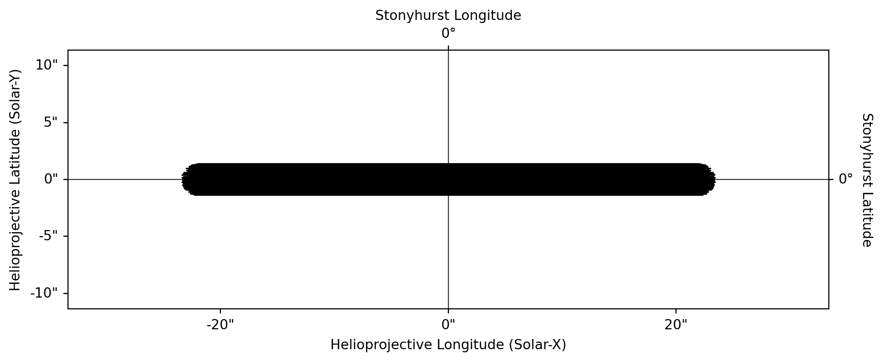
strands = [synthesizAR.Loop(f'strand{i}', c) for i, c in enumerate(bundle_coords)]
bundle = synthesizAR.Skeleton(strands)
bundle.peek(observer=pos)

Toy Loop Model

from synthesizAR.instruments import InstrumentSDOAIA
from synthesizAR.interfaces import RTVInterface

rtv = RTVInterface(heating_rate=1e-3*u.Unit('erg cm-3 s-1'))
bundle.load_loop_simulations(rtv)
print(bundle.loops[0].electron_temperature[0,:5])
print(bundle.loops[0].density[0,:5])

[2657918.14792826 2657918.14792826 2657918.14792826 2657918.14792826
 2657918.14792826] K
[1.71435745e+09 1.71435745e+09 1.71435745e+09 1.71435745e+09
 1.71435745e+09] 1 / cm3

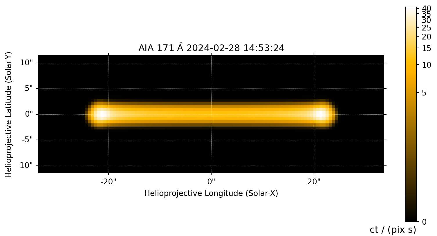
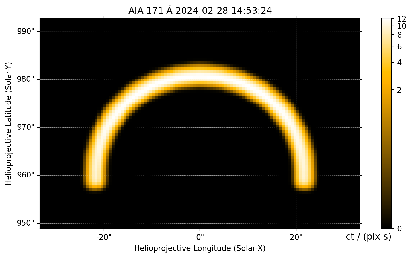
aia = InstrumentSDOAIA([0, 1]*u.s, pos, pad_fov=(10, 10)*u.arcsec)
maps = aia.observe(bundle, channels=aia.channels[2:3])
maps['171'][0].peek()

Toy Loop Model: Summary of Steps

1. What structures are emitting–synthesizAR.Skeleton, synthesizAR.Loop
2. \(T,n\) of these structures as a function of \(s,t\)–synthesizAR.interfaces.RTVInterface
3. How plasma emits as a function of \(T,n\)–synthesizAR.atomic.EmissionModel (optional)
4. How is the emission being observed–synthesizar.instruments.InstrumentSDOAIA

flowchart LR
  coords["SkyCoord
              SkyCoord
          ...
              SkyCoord"]
  loops("synthesizAR.Loop
         synthesizAR.Loop
         ...
         synthesizAR.Loop"):::synthesizar
  skeleton("synthesizAR.Skeleton"):::synthesizar
  modelparams["model parameters"]
  model("synthesizAR.interfaces.RTVInterface"):::synthesizar
  observer["SkyCoord"]
  instrument("synthesizAR.instruments.InstrumentSDOAIA"):::synthesizar
  ions["fiasco.Ion
        fiasco.Ion
        ...
        fiasco.Ion"]
  emmodel("synthesizAR.atomic.EmissionModel"):::synthesizar
  smap(["sunpy.map.Map"])
  coords --> loops
  loops --> skeleton
  model --> skeleton
  modelparams --> model
  skeleton --> instrument
  observer --> instrument
  emmodel -.-> instrument
  ions --> emmodel
  instrument --> smap
  classDef synthesizar fill:#FE7900

Toy Loop Model: Different Observer

side_on_view = SkyCoord(lon=0*u.deg, lat=-90*u.deg, radius=1*u.AU, frame=pos.frame)
aia = InstrumentSDOAIA([0, 1]*u.s, side_on_view, pad_fov=(10, 10)*u.arcsec)
maps = aia.observe(bundle, channels=aia.channels[2:3])
maps['171'][0].peek()

Toy Loop Model: Using a Different Loop Model

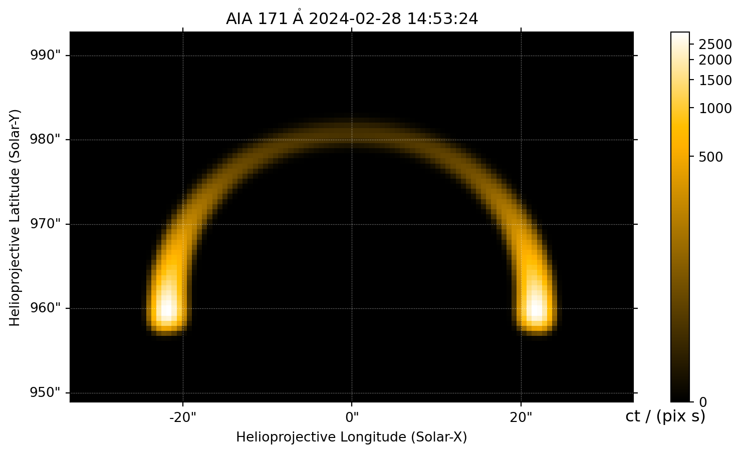
from synthesizAR.interfaces import MartensInterface

martens = MartensInterface(1e-3*u.Unit('erg cm-3 s-1'))
bundle.load_loop_simulations(martens)
maps = aia.observe(bundle, channels=aia.channels[2:3])
maps['171'][0].peek()

Aside: The fiasco Python interface to CHIANTI

• Object oriented approach, HDF5 database, astropy.units everywhere
• Currently only compatible with v8 of the database

import fiasco
temperature = np.logspace(5, 7, 100) * u.K
fe_15 = fiasco.Ion('Fe 15', temperature)
print(fe_15)

CHIANTI Database Ion
---------------------
Name: Fe 15
Element: iron (26)
Charge: +14
Number of Levels: 283
Number of Transitions: 6679

Temperature range: [0.100 MK, 10.000 MK]

HDF5 Database: /Users/wtbarnes/Documents/projects/chianti/database/CHIANTI_v8.0.7/dbase.h5
Using Datasets:
  ioneq: chianti
  abundance: sun_coronal_1992_feldman_ext
  ip: chianti

print(fe_15[0])

Level: 1
Configuration: 3s2
Orbital Angular Momentum: S
Energy: 0.0 eV

print(fe_15.ionization_rate[50:55])

[1.1870807834446956e-12 1.5705204000172247e-12 2.0583888370259458e-12
 2.6732744753822178e-12 3.4411068752377246e-12] cm3 / s

iron = fiasco.Element('iron', temperature)
print(type(iron[14]))
print(iron[14].ion_name)

<class 'fiasco.ions.Ion'>
Fe 15

Toy Loop Model: Advanced Emission Modeling

• By default, InstrumentSDOAIA computes emission using temperature response functions
• Insufficient for: varying abundances, density dependence, time-dependent ionization
• Alternative: compute emissivity of each loop per ion and then integrate over \(R(\lambda)\)
• EmissionModel: select which ions you want to include, temperature range, density range

from synthesizAR.atomic import EmissionModel

ni_14 = fiasco.Ion('Ni XIV', temperature)
fe_9 = fiasco.Ion('Fe IX', temperature)

density = np.logspace(8,12,20) * u.cm**(-3)
em_model = EmissionModel(density, fe_9, ni_14)

em_model.calculate_emissivity_table('emiss_table.zarr')

maps = aia.observe(bundle, channels=aia.channels[2:3], emission_model=em_model)

A Multi-instrument Example

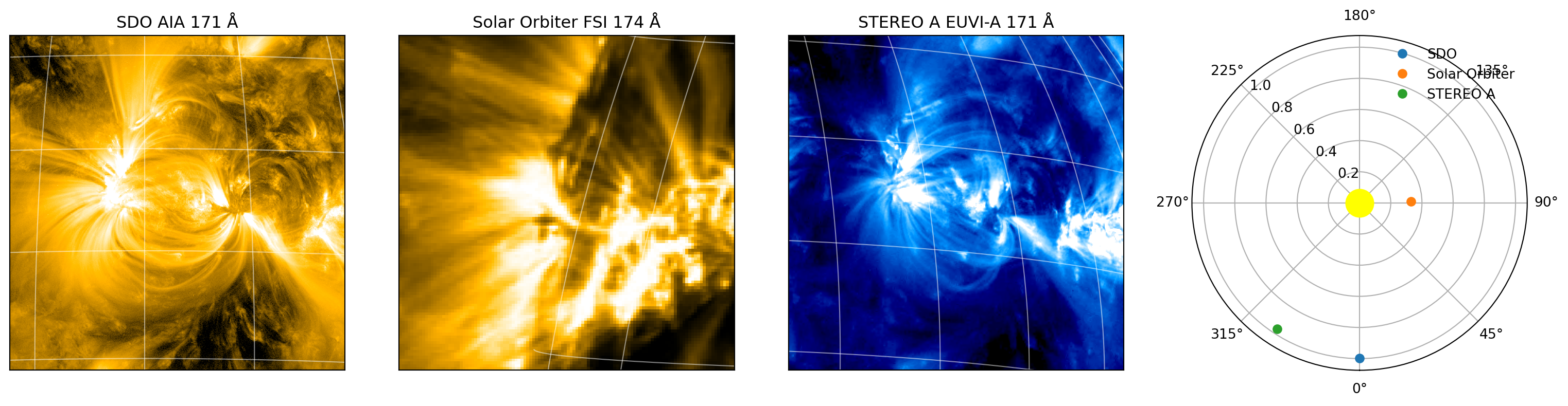
• Active region observed by SDO/AIA, Solar Orbiter EUI, and STEREO EUVI on 2022-03-29 22:50
• AR observed near disk center–use corresponding HMI synoptic map + pfsspy
• Choose only closed loops in range \(20<L<100\) Mm
• Serialize all information about magnetic “skeleton” to asdf

A Multi-instrument Example

skeleton = synthesizAR.Skeleton.from_asdf('data/skeleton.asdf')

skeleton.peek(
  observer=m_eui.observer_coordinate,
  check_visible=True,
  plot_kwargs={'alpha': 0.25},
  axes_limits=(u.Quantity([m_eui.bottom_left_coord.Tx, m_eui.top_right_coord.Tx]),
               u.Quantity([m_eui.bottom_left_coord.Ty, m_eui.top_right_coord.Ty]))
)

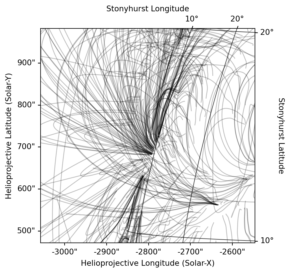
A Multi-instrument Example

from synthesizAR.models.heating import b_over_l_scaling

class MartensCustom(MartensInterface):
    def get_heating_constant(self, loop):
        return b_over_l_scaling(loop, alpha=1, beta=1, H_0=.3e-3*u.Unit('erg cm-3 s-1'))

martens_model = MartensCustom(None, 0.1*u.MK)
skeleton.load_loop_simulations(martens_model)

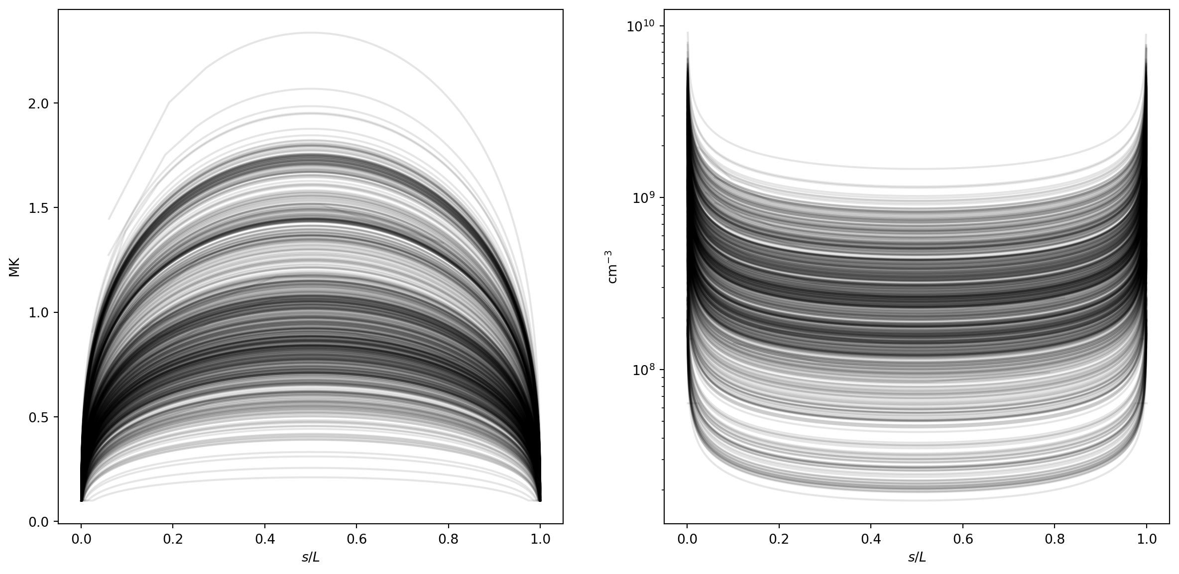
A Multi-instrument Example

class InstrumentSolarOrbiterEUIFSI(InstrumentSDOAIA):
    name = 'SolO_EUI'
        
    @property
    def observatory(self):
        return 'Solar Orbiter'
    
    @property
    def detector(self):
        return 'FSI'
    
    @property
    def telescope(self):
        return 'SOLO/EUI/FSI'

    @property
    def resolution(self):
        return u.Quantity([m_eui.scale.axis1, m_eui.scale.axis2])
    
    def get_instrument_name(self, *args):
        return 'EUI'

• New instruments defined through classes, typically by subclassing InstrumentBase
• Can be as simple as defining new names or complex as defining new ways to compute emissivity
• InstrumentBase defines the expected interface for a new instrument class

A Multi-instrument Example

eui = InstrumentSolarOrbiterEUIFSI([0,1]*u.s,
                                   m_eui.observer_coordinate,
                                   fov_center=m_eui.center,
                                   fov_width=get_fov_from_submap(m_eui))
m_eui_model = eui.observe(skeleton, channels=eui.channels[2:3])['171'][0]

Application: Active Region Heating

See Barnes et al. (2019),Barnes et al. (2021)

Application: EUV Flare Emission

Courtesy Brock Parker and Chunming Zhu (MSU)

Application: Full-disk Stellar Modeling

Courtesy Alison Farrish (NASA GSFC), Farrish et al. (2018)

Summary

• synthesizAR–pure Python package for modeling time-dependent emission from field-aligned models
• Openly developed on GitHub, documentation on Read the Docs, testing on GH Actions
• Takes full advantage of the scientific Python stack + astropy + sunpy
• Prioritizes modularity and flexibility–geometry, loop models, instrument
• sunpy.coordinates + modularity enable multi-instrument modeling studies
• Future: stability, performance, loops with finite width, non-thermal emission

Barnes, W. T., Bradshaw, S. J., & Viall, N. M. 2019, ApJ, 880, 56

Barnes, W. T., Bradshaw, S. J., & Viall, N. M. 2021, ApJ, 919, 132

Farrish, A. O., Maruo, M., Barnes, W. T., et al. 2018, in LPI Contributions, Vol. 2065 (Houston, TX USA), 2043